Background
Adjusting an opt-in sample against a probability reference sample has become routine, and the estimators used to do it are well documented. Two decisions inside that adjustment are not, and both are hard to catch for the same reason: they leave no trace in anything the analyst inspects afterwards. The margins close to numerical precision whichever way they go, the weight file carries no record of how the pseudo-weight was constructed, and the interval looks reasonable.
Survey researchers increasingly work with samples that carry no design weights: opt-in web panels, river samples and volunteer samples. The standard remedy is to borrow structure from a probability reference sample, hereafter the reference, that measures the same covariates. Three estimators are commonly used (Elliott and Valliant 2017; Wu 2022):
-
Inverse propensity weighting models the probability of participating in the volunteer sample rather than appearing in the reference, and weights each volunteer by a function of that fitted probability.
-
Mass imputation fits an outcome model on the volunteers and projects it onto the reference (Kim and Rao 2012).
-
The doubly robust combination uses both, and is consistent if either model is correctly specified (Chen et al. 2020).
These estimators go unrecorded partly because the propensity model, the calibration and the variance usually live in three separate scripts, so no single artifact states what was decided.
The intended reader already weights household surveys and now has to adjust a volunteer source. Illustrations use weightflow (Ferreira 2026), but nothing here is specific to that implementation. nonprobsvy (Chrostowski et al. 2025) implements the same three estimators with analytic and bootstrap variance, and its bootstrap redraws the probability sample according to its declared design. It requires that declared design: replicate weights for the probability sample are not supported, and where an agency releases replicate columns rather than stratum and primary sampling unit (PSU) identifiers, those columns are all one has. It does return a weight vector from a doubly robust fit, but that vector is the inverse-probability weight: applying it to a study variable reproduces the Hájek estimate, not the doubly robust one, which adds the outcome model’s projection for each variable separately. The weight used here carries the doubly robust adjustment itself, so one column serves any study variable.
The Adjustment
Forming the Pseudo-Weight
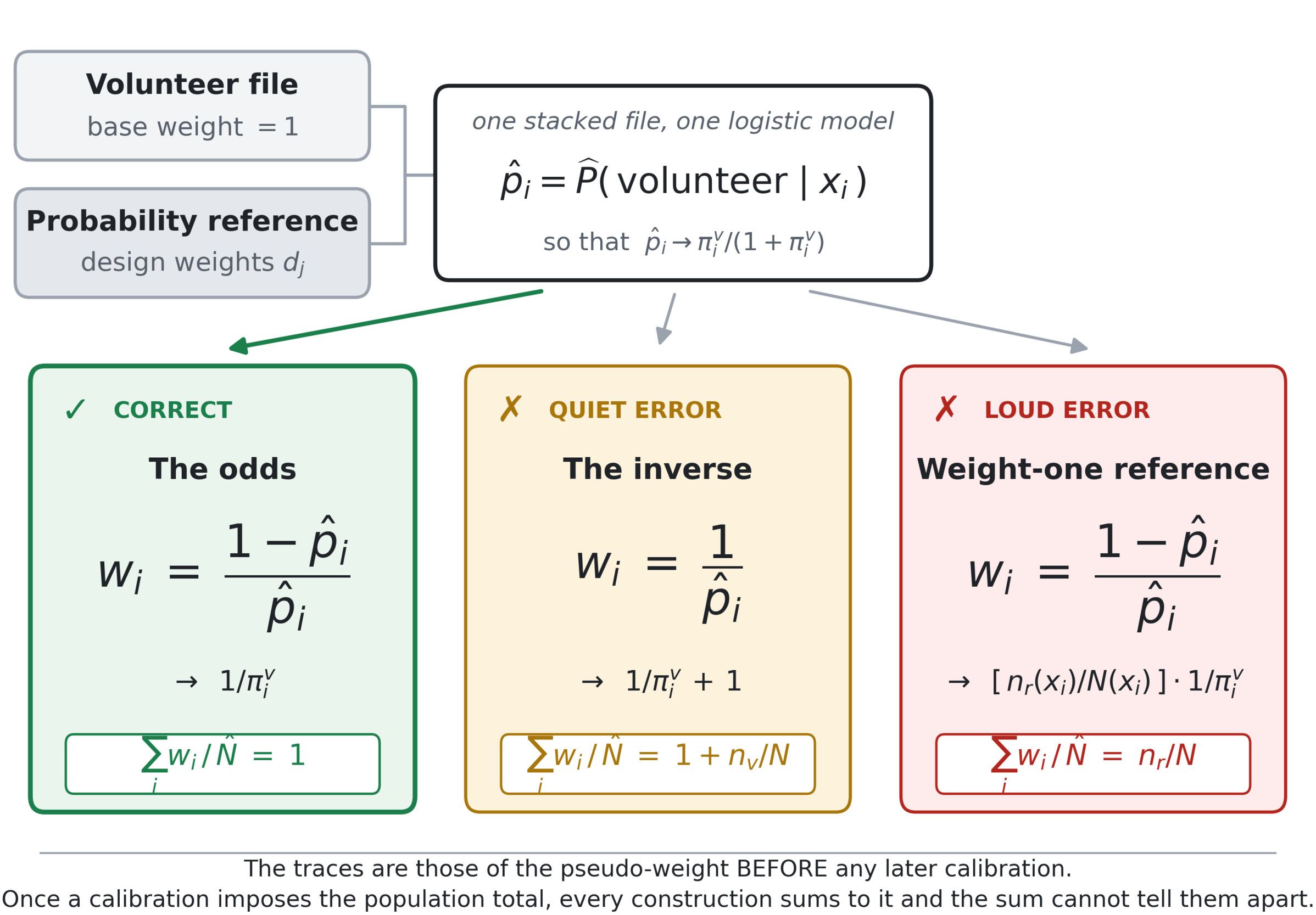
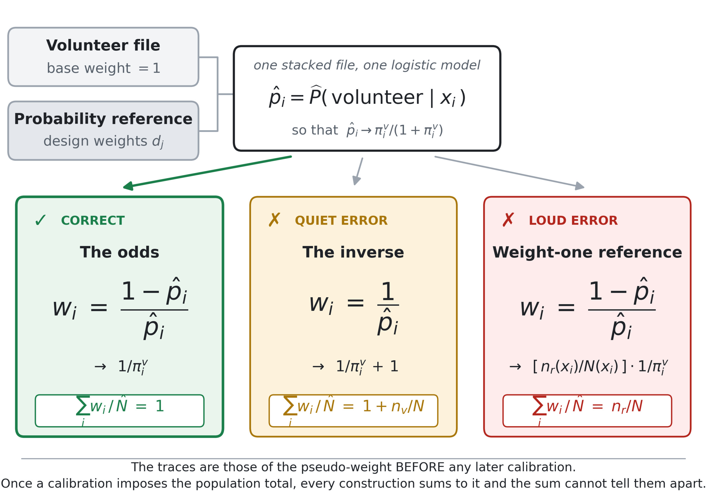
Stack the volunteer file and the reference and fit one model for membership. Two details decide whether what comes out is a pseudo-weight (Figure 1).
Notation. Let index a record of the stacked file; is the fitted probability that record comes from the volunteer file rather than the reference, the unknown probability that population unit participates, which is what the adjustment must recover, its pseudo-weight, and the design weight of reference unit Write for the population size, for the number of volunteers, for the number of reference units, and for the reference’s estimate of so that is the sum of the pseudo-weights relative to that estimate.
First, the reference enters with its design weights, not with weight one. Represented that way, the reference block stands for the population rather than for the sample itself, so the model is fitted against the population.
Second, the volunteer’s weight is the odds against having volunteered:
\[w_{i}\ = \ \frac{1\ - \ {\widehat{p}}_{i}}{{\widehat{p}}_{i}}\]
and not the inverse The numerator is the estimated chance that the record came from the reference rather than the volunteer file, and the reason to prefer it is arithmetic. Under the stacking above the volunteer block contributes weight at a given covariate value against the reference block’s so tends to and the odds return exactly. Hence the pseudo-weights sum to the estimated population size, a property worth checking (Valliant and Dever 2011), and worth checking before any later calibration, since once a calibration has imposed the population total the weights sum to it whichever construction produced them.
The same arithmetic says what the two common alternatives return. Taking returns one extra unit of weight per volunteer, so the weights overshoot the population size by exactly and the estimate is pulled towards the unadjusted mean by Stacking the reference at weight one instead returns writing and for the reference count and the population size at covariate value so the factor is the reference’s own sampling fraction there. It is constant, and harmless, when the reference is self-weighting, but varies across its design strata when it is not, so those fractions enter the fitted propensity score as though they were participation behaviour.
Table 1 runs all three on the same fitted model. Both errors are small next to the unadjusted mean’s 7.4 percent bias, but they are not equally dangerous. The weight-one variant is the larger, at 0.75 percent, and calibrating on age and sex removes almost none of it, leaving 0.72; adding region, which defines the reference’s design strata, absorbs it, to −0.20 against the odds construction’s −0.17, and with a self-weighting reference it does not arise at all, giving −0.08 against −0.05. The inverse is the opposite case: its additive discrepancy is the smaller of the two here, and calibrating on age and sex attenuates it substantially, from +0.22 to −0.06. That attenuation is empirical, not an algebraic identity: the construction still differs from the target pseudo-weight by one unit per volunteer whatever the margins. Before calibration it leaves only a small trace, its pseudo-weights summing to 1.045 times the estimated population size against the odds construction’s 1.001; after calibration that trace is gone from the weight sum. The practical order is therefore the reverse of the apparent severity: the loud mistake is the one that can be diagnosed and, in this design, absorbed by calibration on the reference’s design strata.
Two assumptions underlie everything that follows, and neither is free: selection must be ignorable conditional on the adjustment covariates, and positivity must hold, so that every unit has a non-zero probability of participating. The computational steps are straightforward; the inferential assumptions are not.
The Simulation
A population of carries age, sex, region and two continuous covariates. Participation is logistic in observed covariates at a rate of 4.4 percent, giving volunteer samples averaging about 2,640, so the finite population correction is negligible for the comparisons that follow. The reference is a stratified simple random sample of drawn by region, allocated in proportion to the square root of the stratum size, so its design weights range over a factor of 1.8 and it is not self-weighting; it carries those weights and its replicate columns. Reference units are removed from the volunteer file, and the outcome is non-linear in one covariate, which a linear working model cannot capture.
A fourth covariate enters no model anywhere in the study and its population mean is taken as known, playing the part of a held-out population benchmark: a figure the weighted file can be tested against precisely because the adjustment was never asked to reproduce it. It is correlated with the unobserved driver used below, and is reported as a z statistic on Kish’s effective sample size.
Working models are regression trees with three-fold cross-fitting; the participation model is logistic. The margins calibrated exactly are age and sex; the models use those plus region and the two continuous covariates. The asymmetry is deliberate: region defines the reference’s own design strata, so calibrating on it would mask one of the two errors under study. Monte Carlo draws with bootstrap replicates that re-execute the entire adjustment, seed 20260911. Every randomised step inside a draw, the cross-fitting folds and the bootstrap’s resampling pattern alike, is seeded from the draw, which makes the two arms of Table 3 comparable. The Monte Carlo error of a coverage figure is about 1.5 points, and 2.2 where
What the Reference Contributes
Do the Adjustments Work?
Table 2 gives the baseline. Unweighted, the volunteer mean is 7.4 percent too high and the nominal interval covers nothing. All three adjustments remove almost all of it. The doubly robust adjustment weight used here is the best centred, at −0.01 percent, and inverse propensity weighting is the one at nominal coverage; the other two miss it in opposite directions.
The variance estimates range from close to nominal to conservative for all three, with ratios between 1.04 and 1.30, and the two departures from nominal coverage follow. Mass imputation under-covers at 0.925 because a correctly sized interval around a displaced centre covers less than a nominal one, and the doubly robust weight over-covers at 0.995 because its variance is the most conservative. An interval wider than it needs to be is not an error, but should be reported as such.
The resulting weights show no obvious pathology: the margins close to within the design effect has median 2.36, no unit receives a negative weight, and the held-out benchmark is met at +0.02 standard errors.
Does It Matter Whether the Reference Sample’s Sampling Variability Is Propagated?
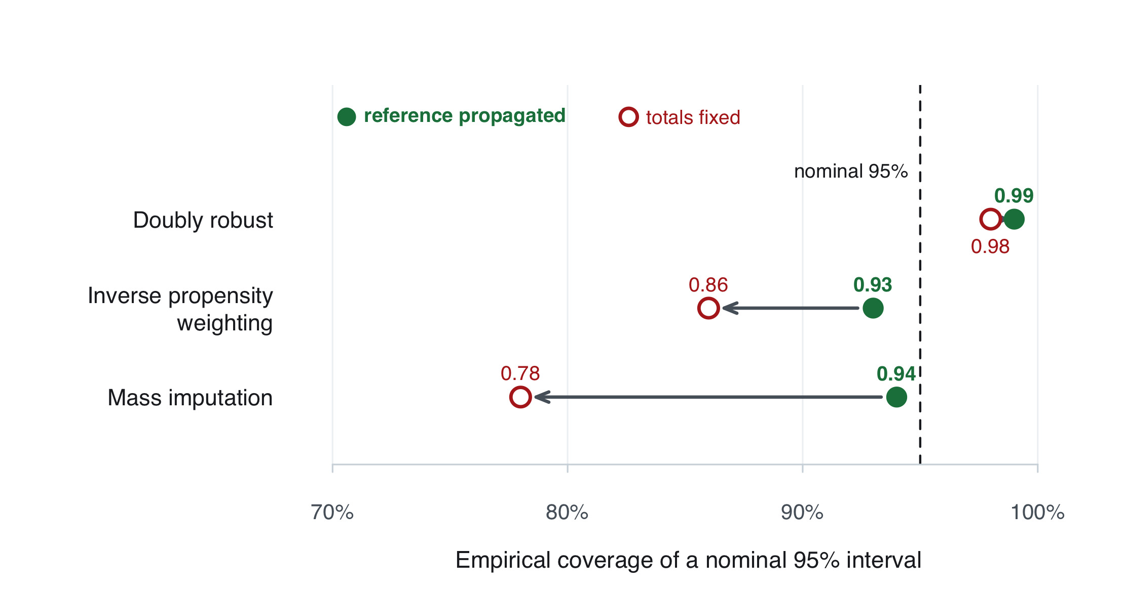
The control totals the model-assisted component reproduces are estimated on the reference, and whether that survey’s own variability enters the standard error is one argument: the reference is supplied with, or without, its own replicate weights. Table 3 and Figure 2 run the same draws twice, differing in nothing else; in both arms the propensity-score and working models are re-fitted on every replicate.
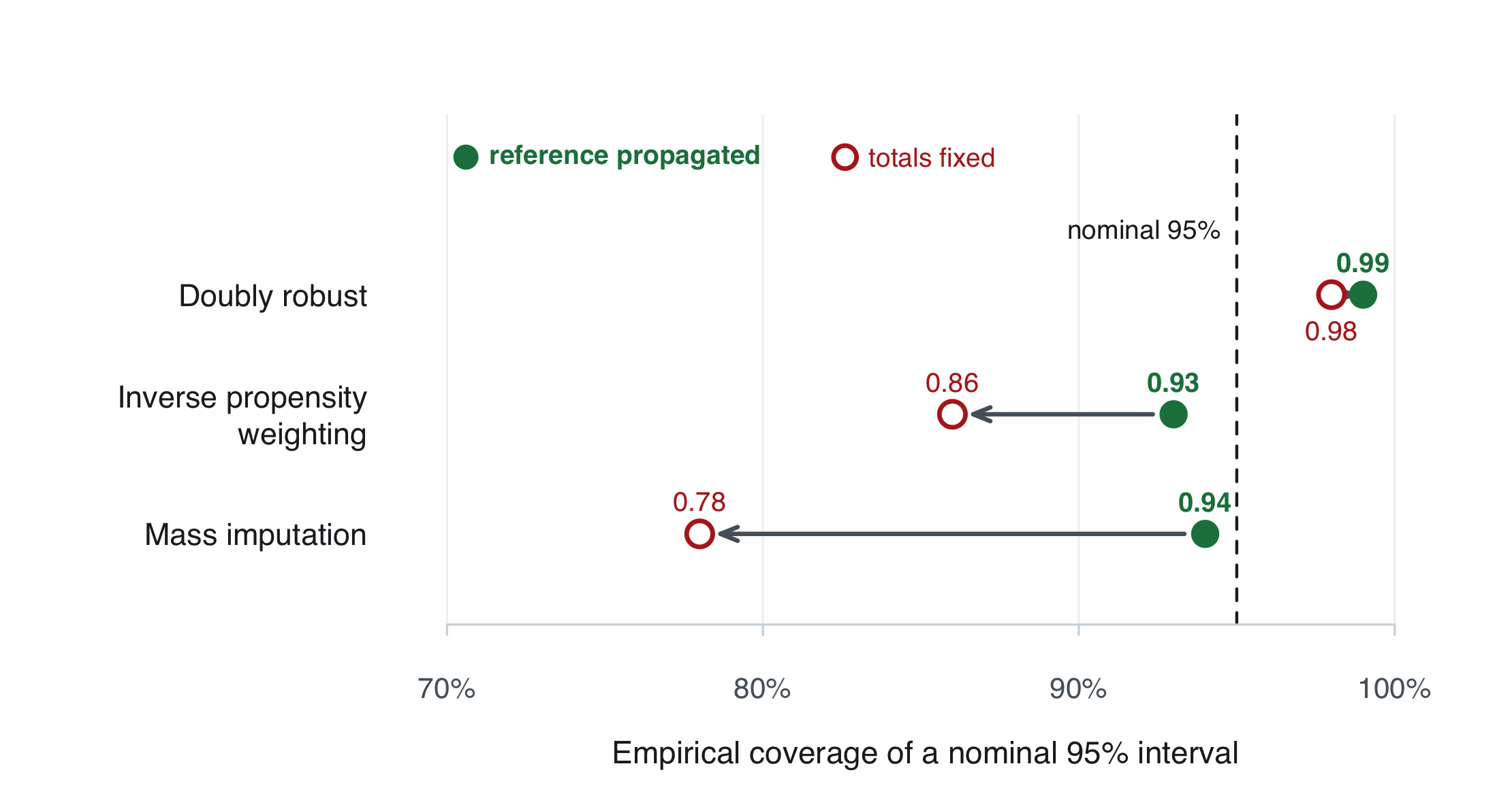
Holding the totals fixed divides the estimated standard error by 1.35 for mass imputation, 1.30 for inverse propensity weighting and 1.29 for the doubly robust weight, but the consequence for coverage depends on how much slack the variance had. Mass imputation falls from 0.94 to 0.78; the doubly robust weight barely moves, from 0.99 to 0.98, because its propagated variance was conservative enough to absorb the loss. Understating the reference’s contribution is therefore most consequential where the variance was otherwise well calibrated.
The magnitude is specific to this ratio of reference to volunteer sample and narrows as the reference grows; the direction does not change, since treating estimated targets as fixed omits a non-negative component of the variance.
When Ignorability Fails, Does Anything Warn You?
We repeated the design with participation additionally driven by a variable no adjustment observes, the situation panel research documents routinely (Thornton and Dejesus Lina 2026). Table 4 reports what happens.
The adjustments remove roughly half of the naive bias and leave 4.2 to 5.3 percent, and coverage falls to between 0.0 and 1.5 percent. The variance estimates range from close to nominal to conservative throughout, so the collapse in coverage is driven by bias rather than understated variance.
The ordering changes sharply. Under ignorable participation the doubly robust weight was the best centred and mass imputation the worst; here mass imputation is the least biased, at 4.21 percent, and the doubly robust weight is indistinguishable from inverse propensity weighting alone, 5.27 against 5.28, well inside the Monte Carlo error of 0.06 points. Combining the two buys nothing: the working model learns a conditional mean itself displaced by the unobserved driver, and weighting it by an equally displaced propensity score returns the propensity estimator’s bias. Double robustness protects against misspecification of either model given ignorability, not against its failure.
No diagnostic computed on the weight would have warned the analyst. The margins close to in both scenarios, no unit receives a negative weight in either, and the design effect is if anything lower under non-ignorable participation, with median 2.04 against 2.36. That is not an accident of these particular statistics: a diagnostic built from the weights and the covariates behind them cannot detect a dependence on a variable absent from both.
The held-out benchmark does warn. Against a population quantity the adjustment was not asked to reproduce, the weighted file is off by 22.8 to 24.9 standard errors under the broken mechanism, against 0.02 under the ignorable one, and the benchmark detects the failure in 100 percent of draws against 7. Holding a margin out in order to test against it costs precision there, but the alternative is a weight whose only evidence of validity is that it reproduces what it was told to reproduce.
Conclusion
Two decisions inside a routine adjustment are worth recording rather than leaving to the default, and a third question is worth asking of any diagnostic.
Record how the pseudo-weight was formed. The odds construction with a design-weighted reference recovers the target pseudo-weight under the stacking used here. The distortion from stacking the reference at weight one can be absorbed when the reference is self-weighting or when the calibration margins span its design strata. Using the inverse adds a unit of weight per volunteer, so its discrepancy in the pseudo-weight is proportional to the volunteer share of the population and becomes smaller as that share falls. The check that distinguishes the three constructions is essentially free, but the ordering matters: before any calibration, the pseudo-weights should sum to the estimated population size, and the comparison has to be made to three significant digits, since afterwards that total holds by construction.
Account for the reference sample’s sampling variability, or state that you did not. Where the producing agency releases replicate weights with the file, those columns carry the reference’s design and can be taken through the whole adjustment. Where it does not, they can often be reconstructed if sufficient information on the reference’s design is available. What should not be left unstated is that the reported standard error treats the estimated totals as known, because nothing inside the calculation reveals the omission, and it is least visible in the estimator whose interval was already the widest.
Hold something out, because the weight diagnostics cannot see selection bias. Kish’s design effect is a property of the weights and says nothing about whether the weighted sample resembles the population. In the scenario here the weight diagnostics look fine and the margins close to numerical precision even though selection bias remains, and that is structural rather than a shortcoming of any particular statistic. A benchmark the adjustment did not use can see it, and here it does by a wide margin. Reserving one known population quantity for that purpose is the cheapest available protection; the data-defect diagnostic (Meng 2018) is another.
One result qualifies a common motivation for using the doubly robust estimator. The doubly robust weight is the best centred when participation is ignorable and no better than the propensity weight alone when it is not, while mass imputation is the worst in the first case and the least biased in the second. Neither ordering is a defect of either estimator. But a practitioner choosing on the strength of a robustness label should know that the label is conditional, that the condition is the one assumption nothing in the data can check, and that the ordering changes sharply across it.
These checks are available at all because the adjustment lives in the weight rather than in an estimator formed separately for each variable: the weight can be inspected and its sum read before any estimate is published.
Availability
Every result was produced with weightflow 1.3.0 under R 4.5.1; the seed is 20260911 throughout. The simulation script, the script that generates every table and every number quoted in this article from the stored results, the raw per-configuration output, a manifest mapping each table to the named configuration that produced it, and checksums of all of it are deposited at https://doi.org/10.5281/zenodo.22736077 . Each table is reproduced by a single command with the configuration named in the manifest; nothing in the script is edited between configurations, and no number in this article is transcribed by hand.
Conflict of Interest
The author is the developer of weightflow, the R package used for the illustrations in this article. Every empirical claim here rests on synthetic populations whose estimands are known independently of any weighting, and the deposited script reproduces all of them; the estimators, the variance principle and the bootstrap are not the package’s contribution, and the functional differences from the alternatives are stated in the text. Part of the material in Table 3 is established, for a weight shared across several study variables, in a manuscript by the author currently under review; the extent of that overlap is set out in the accompanying response to the reviewer.
Corresponding Author Contact Information
Juan Pablo Ferreira, Facultad de Ciencias Económicas y de Administración, Universidad de la República, Montevideo, Uruguay. juanpablo.ferreira@fcea.edu.uy