What are Classification and Regression Trees and How are They Constructed?
If you have ever used the popular chi-square automatic interaction detection (CHAID) (Kass 1980) method for predicting survey response or other market segmentation, you have been building tree-based models. Classification and regression trees (CARTs) (L. et al. 1984) represent another type of tree-based method for classification or prediction. Like CHAID, CART models can be applied to both categorical outcomes as well as continuous outcomes, but CART models extend the capabilities of CHAID models by allowing both categorical and continuous predictors.
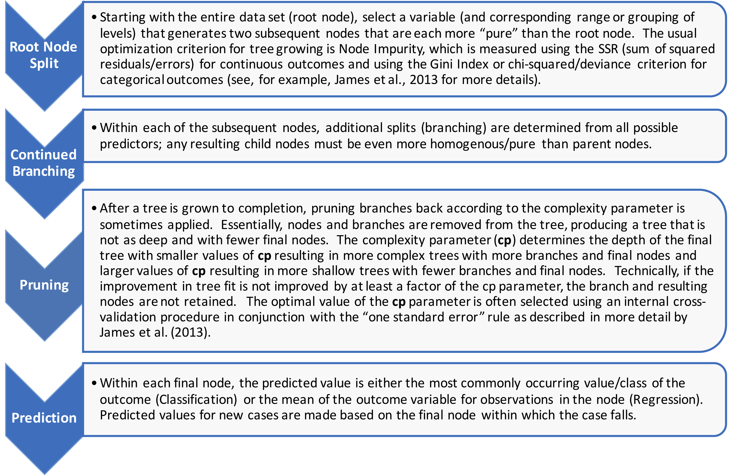
Beginning with the entire dataset (also called the root node), CART models use a series of recursive binary splits based on evaluating every possible predictor to create partitions of the sample into more homogeneous subsets or nodes. Unlike CHAID analyses that utilize statistical tests of association, CART models evaluate and base splitting and node formation on a degree of homogeneity based on the deviance score or Gini index (see James et al. 2013 for more details) for categorical outcomes and the sum of squared errors for continuous variables. For categorical outcomes, the tree models use a “classification tree,” and the predicted value for any case within a particular final node is simply the most commonly occurring level in that final node. On the other hand, if the outcome variable is continuous, then the tree models use a “regression tree,” and the predicted value for any case falling within a particular final node is computed as the mean of the outcome variable for cases in that final node. CART models require specification of a single tuning parameter, which essentially determines the complexity of the resulting tree often referred to as cp. The cp parameter specifies the factor by which further splitting of the tree improves the overall measure of homogeneity. Larger values of cp result in shallow trees with fewer final nodes, while smaller values result in deeper trees with more final nodes. Setting the value of cp essentially controls the amount of pruning that happens for an otherwise fully grown tree. Pruning or trimming a tree is a critical step in the final tree model as it controls the amount of overfitting that is tolerated. More specific details regarding the steps taken to construct CART models are provided in Figure 1. Popular packages for implementing classification and regression trees in R are highlighted in Table 1.

Advantages and Disadvantages of Classification and Regression Trees
One of the most appealing aspects of CART models is that once constructed they can be plotted and resemble real “upside” down trees with a root node at the top and the branches and final nodes (or leaves) at the bottom of the plot. The visual nature of the tree can also be translated into a series of steps or rules that can be used to make predictions. However, tree models do have the potential for overfitting, resulting in estimates with little bias but higher variance. Other major advantages and disadvantages are summarized in Table 2.
How Have CARTs Been Used in Survey Research?
The application of CARTs to various aspects of the survey process has grown steadily in the past decade. For example, McCarthy and Earp (2009) used classification trees to investigate factors related to survey reporting errors. Garber (2009) used classification trees to predict eligibility of units included in a master mailing list for a survey targeting farms. Burgette and Reiter (2010) use regression trees as part of a multiple imputation strategy for continuous health-related survey outcomes such as birth weight. Phipps and Toth (2012) applied regression trees to data from the Occupational Employment Statistics Survey to estimate response propensities for sampled establishments. They also used a second regression tree to examine the potential of nonresponse bias in reported wages.
What are Random Forests Models and How are They Constructed?
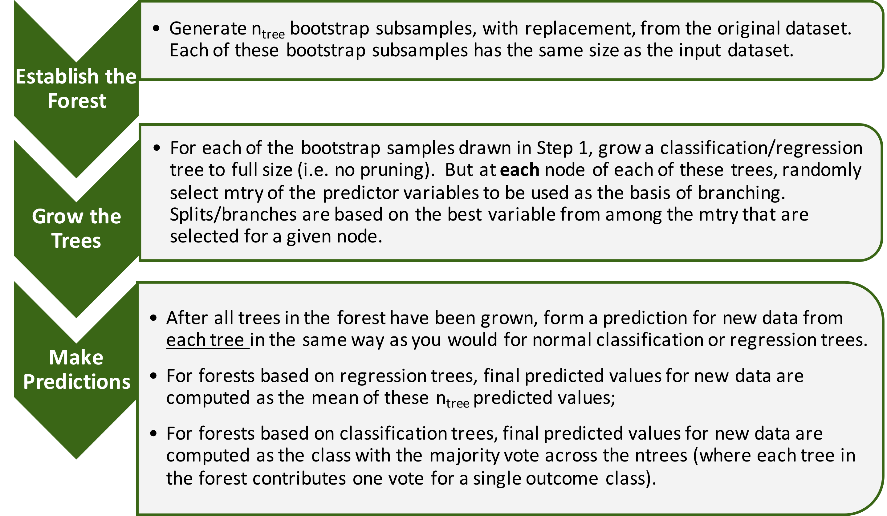
Developed by Breiman (2001), random forests are ensemble-based methods that generate estimates by combining the results from a collection (i.e., the ensemble) of classification or regression trees. More specifically, if the outcome of interest is continuous, then a random forests model produces an estimate of the outcome by averaging the estimates derived from a series of regression trees. On the other hand, if the outcome is binary, a random forest generates an estimate defined as the level that is predicted most often among a collection of classification trees. By combining results across an ensemble of trees, random forests avoid the overfitting tendency of any single tree and generate predictions with lower variance compared to those obtained from a single tree (Breiman 2001; James et al. 2013). Each tree in the forest is grown using an independent bootstrap subsample that is the same size as the original dataset and selected with replacement from it. While not as commonly used for this purpose, response propensities can be estimated from random forests as the fraction of trees in the forest that predict a returned survey for a given address (see, for example, Buskirk and Kolenikov 2015). We note that the more common approach with binary outcomes is for the random forests to generate an estimated class for each sampled case (e.g., respondent or not).
Splitting each tree in the forest occurs one node at a time, and each tree is grown as large as possible. The number of variables considered for splitting is restricted to a random subsample of all possible predictor variables and represents the first tuning parameter for random forests. The size of this subsample is the same for each node and each tree, and is generally referred to as “mtry.” Large values of mtry result in more correlated trees, reproducing the overfitting behavior that is typical for single trees. The most commonly used value for mtry that balances error with predictive power for classification is the square root of the total number of predictor variables rounded down to the nearest whole number and p/3 for regression with p predictors (Breiman 2001). Apart from mtry, the other tuning parameter is the number of trees to be included in the forest. In practical applications, this value typically ranges from 100 to 1,000, with more trees providing more accurate and more stable estimates at the expense of computing time. For continuous outcomes, there is one additional parameter called node size, which determines whether additional splitting on a node can occur or not. If the number of data points that fall in a node is larger than this threshold, additional splitting occurs; otherwise, the node becomes a terminal node in a given tree. The default value for node size for trees within forests applied to continuous outcomes is 5.
The overall prediction error of the random forest is generally a nonincreasing, bounded function of the number of trees, meaning that after a certain number of trees, the additional reduction in error from adding additional trees to the forest becomes negligible (Breiman 2001). However, it is also completely possible for a smaller forest to produce similar accuracy rates as a larger forest (Goldstein, Polley, and Briggs 2011). While the value of mtry can impact the overall prediction accuracy of the forest, studies have indicated that the overall results tend to be fairly robust with similar performance being achieved across a fairly wide range of values (Pal 2005). For continuous outcomes, it has been shown in practice that prediction error rates can be reduced by using larger values of the node size parameter beyond the default (Segal 2004). More details about random forests construction are provided in Figure 2. Popular packages for implementing random forest models in R are highlighted in Table 3.

Advantages and Disadvantages of Random Forest Models
As mentioned previously, the fact that random forests create estimates by aggregating over a series of trees generally implies less overfitting than a single tree model. Moreover, since random forests are grown based on bootstrap subsamples taken with replacement, they produce an internally valid and nearly unbiased estimate of performance. However, unlike tree models that are easy to visualize, random forests are not easily visualized. However, they can produce a ranking of variable importance for each possible predictor that can easily be displayed graphically. Other major advantages and disadvantages of random forests are provided in Table 4.
How Have Random Forests Been Used in Survey Research?
The use of random forest models in survey research has not been as common compared to tree-based models, but their use has steadily been increasing within the past 5 years. For example, Caiola and Reiter (2010) illustrated how random forests could be used to generate partially synthetic categorical data using data from the 2000 U.S. Current Population Survey. Buskirk, West, and Burks (2013) investigated the use of random forests for estimating response propensities, which were then applied to sampled units on subsequent cross-sectional surveys at later time points to estimate the propensity to respond. Earp et al. (2014) investigated the use of a random forest-like ensemble of trees for evaluating nonresponse bias for establishment surveys. Buskirk and Kolenikov (2015) compared logistic regression and random forest models for nonresponse adjustments to sampling weights based on propensity scores.
Classification Example
Using the National Health Interview Survey (NHIS) example training dataset, we estimated a main effects logistic regression, classification tree and random forest model to predict the simulated survey respondent outcome based on a set of core demographics as described previously in this paper. The three models were developed using the training dataset and applied to the testing dataset to evaluate various performance metrics including percentage correctly classified, sensitivity, specificity and the area under the ROC curve, and a measure of balanced accuracy — defined as the mean of the sensitivity and specificity measures. The classification tree was computed using a cp value of 0.0022, which was determined using 10-fold cross-validation of the training data along with a one-standard error rule. The random forest model used a total of 1,001 trees based on preliminary testing along with the default value of the mtry tuning parameter.
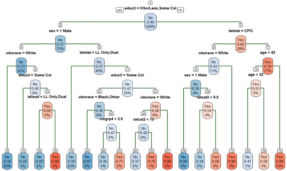
The final classification tree model is provided in Figure 3, and the summary statistics for the accuracy of this model in comparison to the random forest and main effects logistic regression models are provided in Table 5. The final tree model contains 18 final nodes that are shown on the very bottom of the tree in Figure 3. Generally, tree models are read from the top down — if the condition specified at any given node is true, then proceed downward and to the left; otherwise, proceed downward and to the right. Continue making your way down the tree until you reach one of the final nodes. The left-most final node (number 8) represents white males who have less than a BS/BA degree. These individuals comprise 25% of the entire sample, and a minority of these individuals were respondents (16%). A future individual who is male, white, and has less than a BS/BA degree would be predicted to be a nonrespondent using this tree model.

Generally speaking, the random forest model outperformed both the tree and logistic regression models on a majority of the metrics, but both the forest and tree models outperformed the logistic regression model on all metrics. In particular, both the random forest and tree models were more specific than the logistic regression model (i.e., higher correct detection of non-respondents) and had between 7 and 10 percentage points higher sensitivity values (i.e., higher correct detection of respondents). The same spread for the area under the curve was also realized for the forest and tree models compared to the logistic regression model. Since the binary outcome was simulated through a series of probit models involving nonlinear and interaction terms, we would expect lower performance from the main effects logistic regression. In addition, it is important to note that the nonparametric nature of the forest and tree models were able to approximate these more nonlinear and complex probit models and create predictions that had a relatively high level of accuracy and performance without having to specify the shape/structure of the underlying survey outcome model.