Neural Networks for Survey Researchers

What are Neural Networks and How are They Constructed?

Neural networks (also known as artificial neural networks, ANN) are one of the most popular approaches for regression and classification modeling in the machine learning literature in terms of theoretical research and application. For example, neural networks have achieved great success in tasks such as image recognition (e.g., Krizhevsky, Sutskever, and Hinton 2012); optical character and handwriting recognition (e.g., Graves and Schmidhuber 2008); and natural language translation (Sutskever, Vinyals, and Lee 2014). Elsewhere, Google DeepMind’s recent AlphaGo program (Silver et al. 2016) used neural networks in part to defeat the world expert in a game of Go, largely considered to be one of the most computationally difficult games to win due to its exceedingly large number of possible board configurations. Indeed, neural networks are behind the recent explosive growth of deep learning (LeCun, Bengio, and Hinton 2015), where multiple layers of learners are stacked together, each learning a more abstract representation to aid in the overall prediction. For instance, in an image recognition task where the computer needs to classify what types of objects are in an image, one layer might learn where the lines are within an image, whereas another might learn how those lines organize to represent different shapes, and then how shapes organize to represent objects (e.g., books vs. people vs. pets).

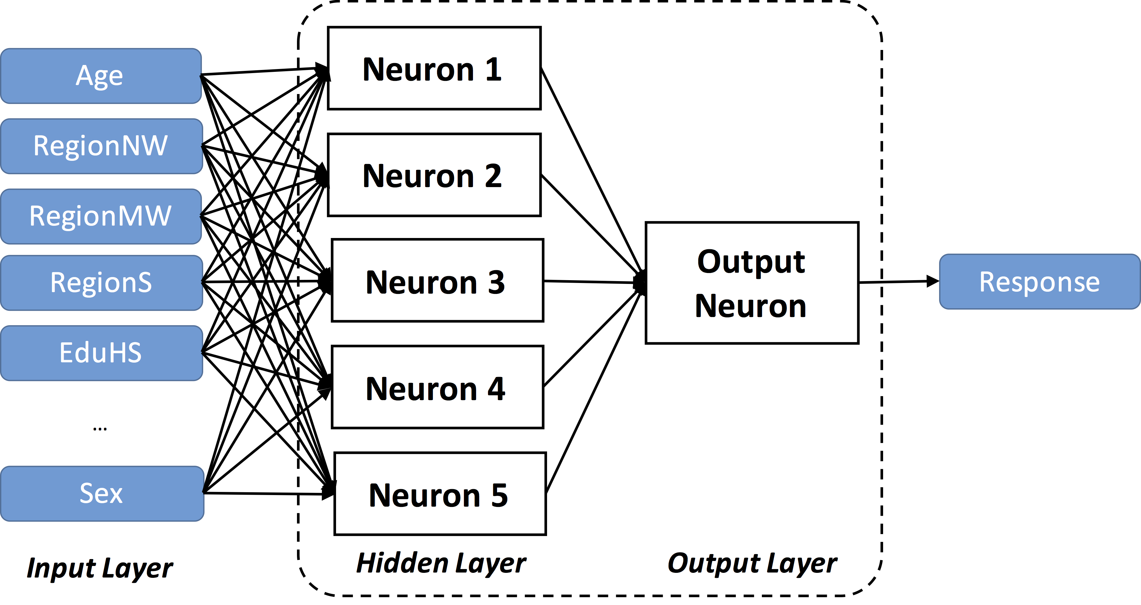
Neural networks are a form of supervised learning that are inspired by the biological structure and mechanisms of the human brain. Neural networks generate predictions using a collection of interconnected nodes, or neurons, that are organized in layers. The first layer is called the input layer as the neurons in this layer only accept variables from the data set as input. The final layer is called the output layer, since it outputs the final prediction(s). Hidden layers refer to those that fall between the input and final layers since their outputs are relevant only inside the network. Neurons create a weighted sum from the input they receive and then transform this weighted sum using some type of nonlinear function such as the logit, hyperbolic tangent, or the rectified linear function. The value computed from the function, operating on the weighted sum, is then passed to neurons in the next layer of the network. Information flows through the neural network in one direction — from the input layer through the hidden layers to the output layer. Once information reaches the output layer, it is gathered and converted to predictions.

Depending on the complexity of the data for which predictions are desired, neural networks may have several hidden layers, and the functions used within the neurons may vary. Theoretically, with enough neurons, one hidden layer of neurons plus an output layer is enough to learn any binary classification task, and two layers plus an output layer can learn a close approximation for any regression task (e.g., Alpaydin 2014, 281–83). In the increasingly popular domain of deep learning, tens of hidden layers might be used to help aid in the discovery of complex, predictive patterns in the data. The overall architecture of the neural network determines which neurons feed their output to other neurons in subsequent layers. Furthermore, the type of variable being predicted governs the number of neurons in the output layer. In particular, for regression tasks (continuous outcomes) and binary classification tasks (dichotomous outcomes), the final output layer consists of a single neuron. Alternatively, for multinomial classification tasks, where there are more than two values in the categorical outcome variable, the final output layer consists of one neuron per possible value. In this case, the predicted class corresponds to the neuron with the highest outputted value. An example neural network is displayed in Figure 1. The network displayed is a so-called “fully-connected network” because each neuron, within each layer, provides input into each neuron in the next layer. We also see from the figure that there is only one hidden layer in the network. Figure 2 provides a more technical description of how neural networks are created and Table 1 highlights a few popular R packages for constructing them.

Figure 1 An example of a fully connected neural network with a single hidden layer. The network takes various demographic variables as input (on the left) to predict a binary response (on the right).

Figure 2 Steps in constructing a neural network.

Advantages and Disadvantages of Neural Networks

One of the most appealing aspects of neural networks is their ability to perform complex classification tasks with high levels of accuracy. Neural networks can improve the results of more traditional classification models, such as logistic regression, by combining the results of multiple models across the layers of the network. The improvements to accuracy do have a trade-off in that neural networks can take more computing time before a final prediction is made. We highlight other major advantages and disadvantages of neural networks in Table 2.

How Have Neural Networks Been Used in Survey Research?

Neural networks are emerging as a useful model for a variety of tasks in survey research literature. For instance, Gillman and Appel (1994) describe the use of neural networks for automated coding of response options (e.g., occupation coding). Nin and Torra (2006) consider the use of neural networks for record linkage (an increasingly relevant task for survey research in the era of Big Data), focusing on cases where different records contain different variables. An advanced type of neural network called recurrent neural networks (RNNs) allow for connections between neurons within a hidden layer that enable RNNs to remember information over time, making them highly useful for sequential data. Eck et al. (2015) have considered the use of RNNs to predict whether a respondent will break off from a Web survey, based on the respondents’ behaviors exhibited in paradata describing their actions within the survey (e.g., navigational patterns between questions and pages, answering and reanswering questions, and scrolling vertically on a page). Recently, these models have also been extended to predict errors at the question level, including predicting whether a respondent will commit straight-lining on a battery of grid questions (Eck and Soh 2017).

Deep learning with neural networks also offers much promise in supporting and augmenting survey-based data collection. For example, sequence-to-sequence models using neural networks (e.g., Sutskever, Vinyals, and Lee 2014) could enable the automated translation between languages spoken by an interviewer and a respondent, removing barriers for data collection from underrepresented populations. Similarly, image segmentation models using convolutional neural networks (e.g., He et al. 2017) could be used to identify objects within smartphone images uploaded by respondents as answers to survey questions (e.g., in food diary surveys) and providing background context paradata to their responses.

Classification Example

Using the National Health Interview Survey (NHIS) example training dataset, we estimated both a main effects logistic regression model and a collection of neural network models for predicting survey response based on a collection of demographic variables. To illustrate how the performance of neural networks can depend on their internal parameters and structure, we constructed a number of neural networks that vary in both the number of neurons used in a single hidden layer^[1] [2, 5, 10, 20, 50, 100], and the number of training iterations ranging from 10 to 200 in increments of 10.

For both prediction tasks, the variables used as input to the neural networks include the respondent’s (1) region, race, education, class of worker, telephone status, and income categorical variables, which were converted into multiple inputs using one-hot coding; (2) Hispanic ethnicity and sex dichotomous variables; and (3) age and ratio of income to the poverty threshold continuous variables that were normalized to a Z score. For evaluating the models (both neural network and logistic regression techniques), 84% of the data was randomly selected for training the models, whereas the remaining 16% was held back as an independent testing data for evaluating the accuracy of the predictions.

The results of our models are presented in Figure 3 and Table 3. From these results, we can make several key observations. First, each of the neural networks with different numbers of neurons in the hidden layer were able to achieve significantly higher accuracy, sensitivity, and specificity after a sufficient number of training iterations than a logistic regression model that trained on the same data. Remarkably, even a neural network with only two neurons in the hidden layer achieved much better performance than the logistic regression, which is notable given that logistic regression is equivalent to a neural network with one neuron. Thus, even a small increase in the complexity of the model can greatly improve predictive performance.

Next, we consider the effects of increasing the complexity of the model, as measured by the number of neurons. We observe that with respect to balanced accuracy (Figure 3b, Table 3), which best^[2] measures combined performance on both positive (response) and negative (nonresponse) data points, that

Figure 3 Predictive performance across training iterations.

increasing the number of neurons generally led to higher predictive performance. Thus, the additional neurons improved the ability of the neural network to learn more nuanced patterns within the data, increasing the ability of the model to differentiate respondents who would ultimately respond versus those who would not. In particular, this result was caused by the networks with more neurons achieving higher sensitivity (Figure 3c, Table 3). This is notable since this implies that the additional neurons were valuable for improving predictions of the less common response outcome, which is indeed more difficult to predict given that there were fewer data points with this outcome from which to learn. However, we also note that the neural network with 50 neurons in the hidden layer slightly outperformed the one with 100 neurons. This could indicate that the model started to become too complex and was beginning to overfit the training data, reducing the generalizability of the patterns it learned.

Finally, considering the number of training iterations, we make two key observations. First, for all of the neural networks, a small number of iterations were needed to outperform logistic regression. Thus, training a neural network model does not necessarily require significantly more computational work than a logistic regression model in order to achieve significant improvements in predictive performance. Second, as the number of neurons in the network increased, a larger number of iterations were required for the model to converge to its best performance. This highlights one of the key trade-offs in neural networks: performance vs. time. That is, the more complex models achieved greater performance at the expense of requiring more time to learn the final, stable model. For smaller problems, such as the data set presented here, the added time expense of increased complexity is relatively small, but for more difficult problems (e.g., with millions of data points or more and with a larger number of possible predicted outcomes), care is often needed to optimally balance this trade-off.