What are Support Vector Machines and How are They Constructed?
Support vector machines (SVMs) are commonly used for classification problems, such as predicting whether or not an individual chooses to vote or whether or not an individual decides to participate in a survey. The first SVM algorithms were developed in the mid-1990s and focused on predicting binary outcomes using machine learning theory to maximize predictive accuracy (e.g., Boser, Guyon, and Vapnik 1992; Vapnik 1995). They have since been extended to solve categorical classification and regression problems (Attewell, Monaghan, and Kwong 2015; James et al. 2013). As an introduction to SVMs in survey research, we focus on SVMs for binary classification.
Like many classification and prediction methods, SVMs classify binary outcomes (e.g., survey response versus nonresponse) by estimating a separation boundary within the space defined by a set of predictor variables. A given observation, defined by the values of the predictor variables — i.e., where it is located in that predictor space — is classified based on which side of the boundary it falls. Theoretically, there are an infinite number of ways such a boundary could be created. In the simplest case, SVMs create a “maximal margin” in the predictor space — the largest buffer separating observations for one outcome from those of the other outcome. Cases that fall exactly on the margin are called support vectors because these specific cases alone define the unique boundary solution. If there are only two predictor variables, the separating boundary is a line; with three predictors, the boundary is a plane; and with more than three predictors, the boundary is typically referred to as a separating hyperplane. Predictions are obtained from SVMs by using the corresponding decision function that is a mathematical depiction of the boundary.
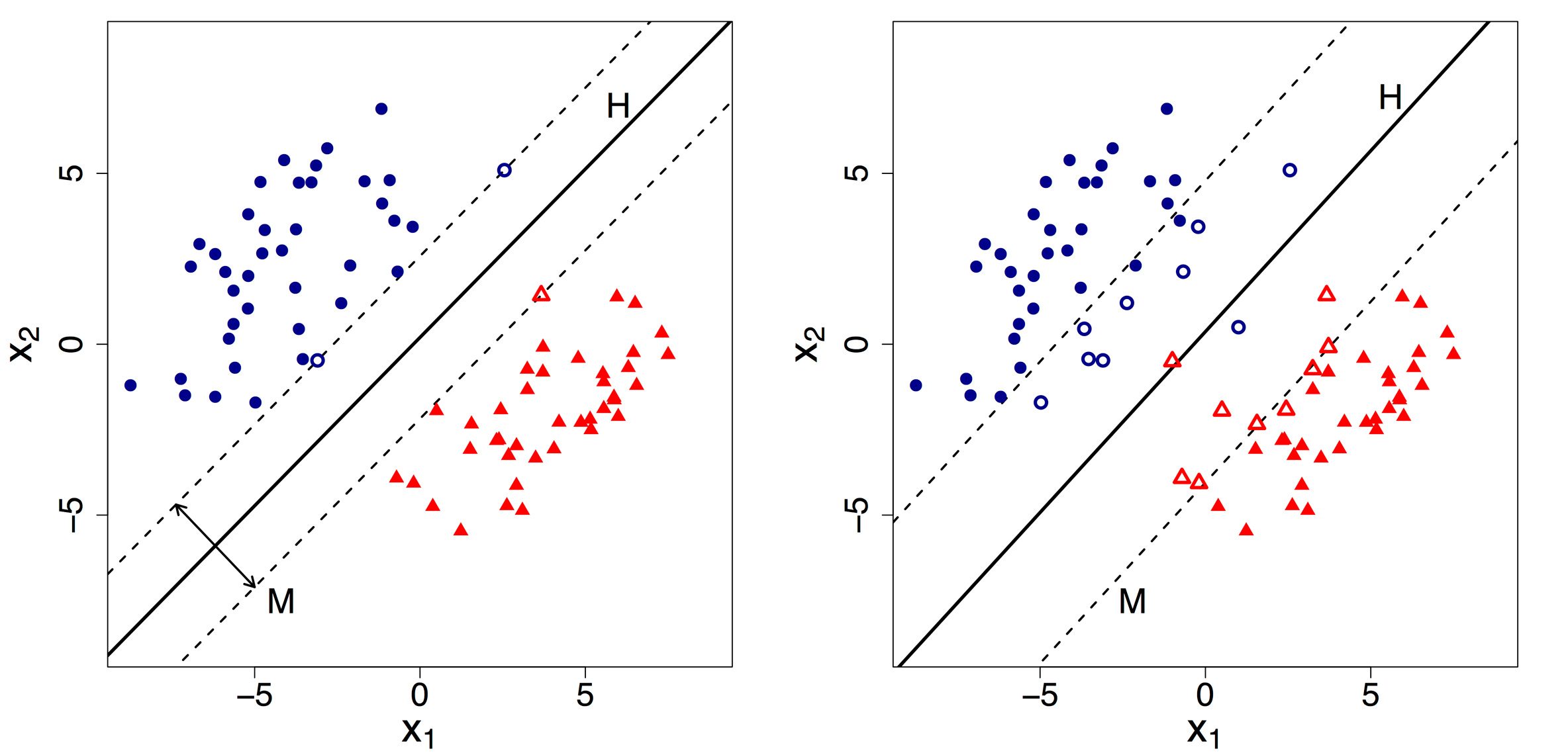
As an example, suppose a researcher wants to predict survey participation based on age (X1) and income (X2). Using these two predictors, the SVM attempts to classify cases as either survey respondents (red triangles) or survey nonrespondents (blue circles), as displayed in the left pane of Figure 1. The optimal hyperplane (i.e., boundary) separating respondents from nonrespondents is the line labeled H. The classification boundary is “optimal” in that it minimizes the classification error in the training data set. In the very simplest case, such as that depicted in the left panel of Figure 1, survey response in the training data is linearly separable by X1 and X2, and the estimated boundary H produces no in-sample classification error. It is easy to see in Figure 1 (left) that one could draw an infinite number of lines that would perfectly classify survey respondents and nonrespondents. This is where the maximal margin comes in. The maximal margin lines are depicted by the dashed lines labeled M. By definition, the separating boundary H bisects the region defined by the margin lines. The maximal margin classifier finds the maximal margins, such that the resulting separating hyperplane H is farthest from the training observations among all such hyperplanes (James et al. 2013). Observations lying along the margin are called support vectors. In Figure 1 (left), these are indicated by the open triangles and open circles. Moving the support vector observations only slightly would alter the margin and the resulting position of the separating hyperplane H. Once the boundary H has been estimated, one can apply it to in-sample (i.e., training) data, to test data, or to new data for forecasting. In Figure 1 (left), observations that fall below the estimated boundary H would be classified as survey respondents, while observations above H would be classified as survey nonrespondents.
_and_nonresponse_(blue_circ.png)
Among the differences in various SVM classifiers, the two that we highlight here are (1) how they deal with classification errors and (2) whether the decision boundary H is a linear versus nonlinear function of the predictors. As the previous example illustrates, in the simplest scenario, we assume that the decision boundary is linear and that it perfectly separates the two outcomes in the predictor space. This assumption — e.g., that survey response versus nonresponse can be perfectly predicted by a linear function of X1 and X2 — usually does not hold in practice. An example of a decision boundary that is not linearly separable is given in the right panel of Figure 1. As can be seen here, no (straight) line exists that would perfectly separate the survey respondents (red triangles) from the nonrespondents (blue circles).
One way to address this issue is to allow for a “soft margin” classifier (James et al. 2013). Contrary to a “hard margin” classifier, the soft-margin classifier allows for (1) observations that are correctly classified but lie between M and H, and (2) misclassified observations — i.e., those that fall on the “wrong” side of H. This technique employs slack variables, which keep track of the margin error for each observation. Finding the optimal boundary H now involves not just maximizing the margin, but also specifying a constraint on the total error T that will be allowed. Sometimes the soft-margin SVM optimization problem is recast to one where, instead of using T, a penalty C is used to weight the error, representing a trade-off between increasing the margin versus reducing misclassification in the training data. The total error T and penalty parameter C are inversely related to the optimal margin. Large penalties C (small allowances T), lead to smaller margins. Smaller penalties C (large allowances T), lead to larger margins, but also more misclassifications in the training data. In practice, the penalty C (or allowance T) is usually set through k-fold cross-validation.[1]
Figure 1 (right), shows an example that is exactly the same as in Figure 1 (left), but with two observations (toward the middle of the plot) that do not allow for linear separability. An SVM model with C=1 (not shown) produces the same margins M and separating plane H as in the left panel. Figure 1 (right) shows the margins and separating plane when C=.01. In this case, there is a smaller penalty for margin violations, so the margins are wider than in the left panel. In addition to observations that lie on the margin, those that fall on the wrong side of their margin are considered support vectors, since changing any of these would change the margin and resulting boundary hyperplane.
_and_nonresponse_(blue_c.png)
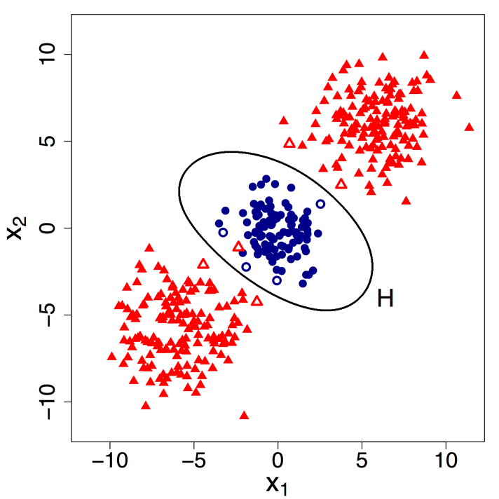
A second issue that arises in SVM classification concerns whether the classification boundary is a linear function of the predictor variables. In Figure 1, it seems reasonable to assume a linear boundary line H. However, the linear assumption is restrictive and may not be appropriate for every application. Figure 2 illustrates the case where survey responses are nonlinearly related to the predictors X1 and X2. It is clear here that no (straight) line can be drawn that reasonably separates respondents from nonrespondents, even if we allow for misclassifications. Most SVM routines now allow for nonlinear transformations of the predictor variables. Typically, one can choose from linear, polynomial, spline, and radial basis functions of the predictors, among others. In Figure 2, we estimated an SVM with a radial kernel and allow for soft margins. Although the data is not perfectly separable even with the nonlinear kernel, we can see that the classification boundary H does a good job of classifying the training data. Any points within the ellipsoid H are classified as nonrespondents. Those outside are classified as respondents. The support vectors are again denoted by open circles and open triangles.
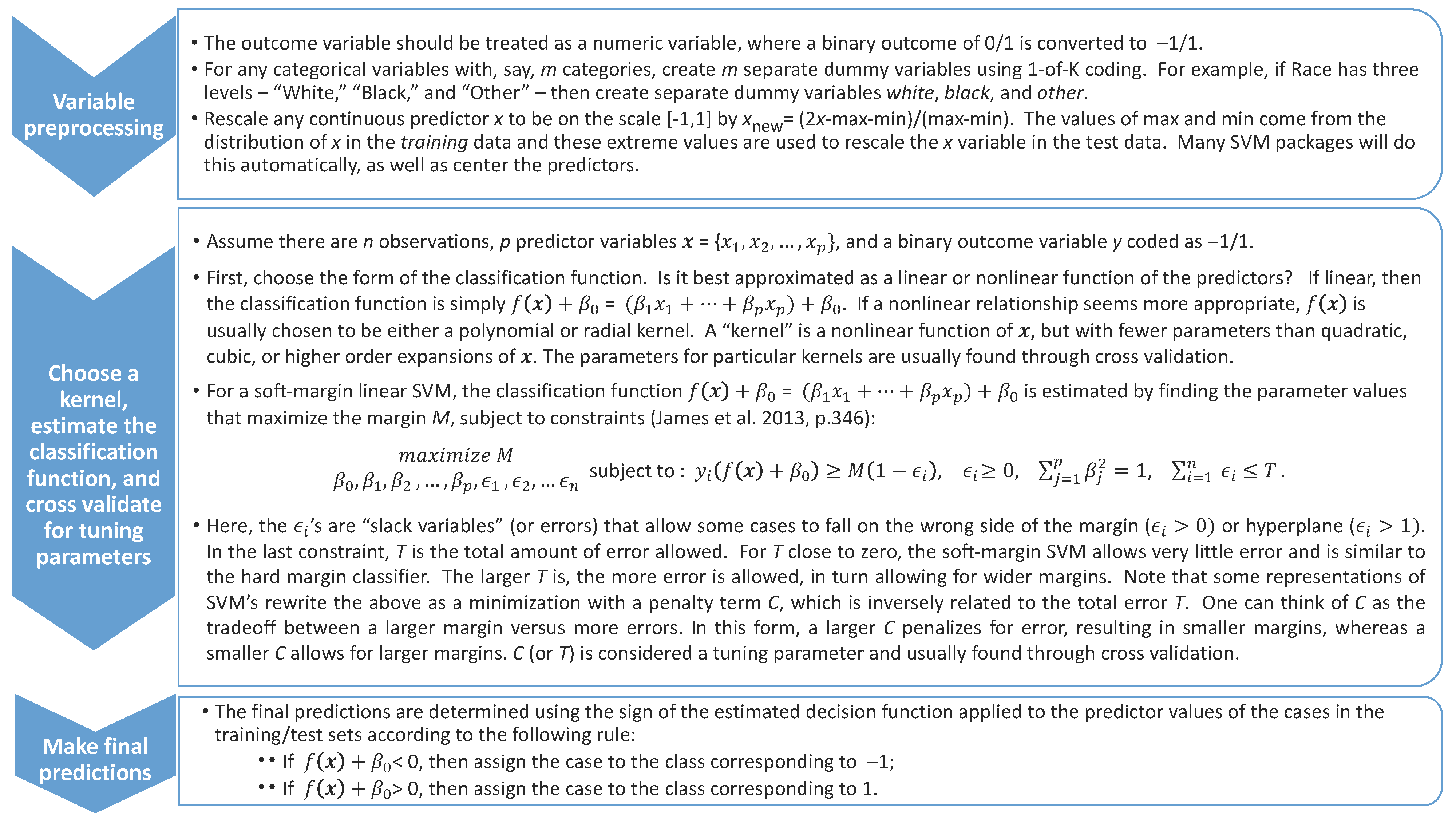
These are just a few simple examples of support vector classifiers/machines. Figure 3 provides more specific details of how SVMs work, including how they estimate the hyperplanes and decision functions, as well as how they can be used to generate predictions. Much of the notation relies on the very accessible introductions to SVMs that can be found in Bennet and Campbell (2000) and in James et al. (2013). An overview of software that can be used for estimating SVMs can be found at http://www.svms.org and http://www.kernel-machines.org/software. A list of R packages that can be used to estimate SVMs can be found at http://www.rdatamining.com. We highlight a few of the more popular R packages that can be used to estimate SVMs in Table 1.

Advantages and Disadvantages of Support Vector Machines
One of the most appealing aspects of SVMs is their versatility. Certainly, SVMs have been successfully applied to a wide range of problems including character recognition and text classification, speech and speaker verification, face detection, verification, and recognition, junk mail classification, credit rating analysis, and cancer and diabetes classification, among others (Attewell, Monaghan, and Kwong 2015; Byun and Lee 2002). However, the versatility of SVMs does not come for free, as these models can take considerable time to run, depending on (1) the number of observations within the data set and (2) the granularity of cross-validation for tuning parameters. SVMs have traditionally been used for binary classification, but recent advances have extended classification to categorical outcomes with more than two classes using one-versus-one or one-versus-all approach (see James et al. 2013 for more details). Despite the extension to multinomial outcomes, SVMs applied to outcomes with more than two classes can be computationally intensive depending on the number of categories of interest and the size of the data sets. We highlight the other major advantages and disadvantages of SVMs in Table 2.
How Have Support Vector Machines Been Used in Survey Research?
While SVMs have gained in popularity, the empirical applications within survey or public opinion research are few. In addition to the applications in other disciplines referenced above, examples include a study conducted by Cui and Curry (2005) that explores the use of SVMs for “robust accuracy” in marketing where the main goal is predictive accuracy rather than structural understanding of the contents of the model. More relevant for public opinion research, Malyscheff and Trafalis (2003) use SVMs for substantive analyses to investigate decision processes in the Electoral College while Olson, Delen, and Meng (2012) investigate bankruptcy using SVMs. Lu, Li, and Pan (2007) have used SVMs for imputation applied to student evaluations and Christen (2008, 2012) for record linkage purposes.
Classification Example
Using the National Health Interview Survey (NHIS) Example training dataset, we estimated two models of survey response: a “typical” logistic regression model – i.e., with no interactions or nonlinear functions of the regressors – and an SVM model. Each included demographic covariates, such as age, sex, race, region of country, income, ratio of family income to the poverty threshold, telephone status, education level, and type of employment. We employed a soft-margin SVM with a radial kernel. To determine the SVM tuning parameter C and radial kernel tuning parameter γ, we conducted 10-fold cross-validation applied to the training data. The resulting cross-validated values for these parameters were γ = 0.0189 and C = 32. The predictors were also preprocessed by centering them and scaling them as illustrated in the example R code displayed in the supplemental materials.
Table 3 presents the confusion matrix for predicting response status computed by applying both the logistic regression and SVM models to the test data. The correctly classified cases fall along the main diagonal of the confusion matrix, while the misclassified cases fall along the off-diagonal. As can be seen from Table 3, both models correctly predicted the response status for the majority of cases.
As indicated by the various performance statistics presented in Table 4, the SVM model outperforms the main effects logistic regression model considerably. Specifically, the SVM model correctly classifies 78% of all cases compared to only 70% for the logistic regression model. Table 4 also shows that the true positive rate is considerably higher for the SVM model (62.9%) compared to the logistic regression model (49.6%). Smaller differences between the true negative rate were noted between the two models with the SVM model correctly classifying 88% of the nonrespondents compared to 83% for the logistic regression model. The overall area under the ROC curve was a full 10 percentage points higher for the SVM model compared to the logistic regression model as well.
Readers should be aware that the letter “C” is frequently used in various SVM articles, books, tutorials, and statistical packages to represent both of the tuning parameters T and C mentioned above. This can be confusing, because the total error T and the penalty C are inversely related in their effect on the estimated margin. As an example, James et al. (2013, 112:346) use C to represent the total “budget” for errors (which we denote as T). On the other hand, the R kernlab package, which we use for our analysis and highlight in Table 1, uses C to represent the penalty for errors. Because the SVM optimization problem can be presented in two equivalent ways, but with inversely related tuning parameters, researchers applying (or reading about) SVMs should be particularly careful in determining which specification has been used and how to interpret the tuning parameter in that context.