Introduction

The main objective of sampling is to obtain a representative sample for an unbiased and efficient estimate within a budget constraint. In a balanced sample, according to Yates’ definition (Yates 1971), the mean value of the balanced factor in the sample is equal to the mean of the factor in the population. In this study, a balanced sample is not a purposively selected sample but a randomly selected one. Another important reason for a balanced sample is to protect the inference against a model misspecification (Royall and Herson 1973a, 1973b). Several approaches including a systematic selection method for a balanced sample have been proposed and practiced (Deville and Tille 2004; Valliant, Dorfman, and Royall 2000).

Research Objective

In this work, we propose and demonstrate a practical balancing method which would be a small modification to currently practiced design-based sampling procedures for small and large-scale surveys. Consider the problem of selecting size n sample from a population of N elements. There would be 49,950 ways to select a size 2 sample from a population of 1,000 elements. The simple random sampling procedure would give an equal chance to each of the potential 49,950 samples. With a systematic selection procedure (Cochran 1977; Kendall, Stuart, and Ord 1983; Sarndal, Swensson, and Wretman 1992), there would be 500 possible samples of size 2 from a population of 1,000 ordered elements. There would be 6.3851×10139 potential simple random samples of size 100 from a population of 1,000 elements! Meanwhile, there would be only 10 possible systematic samples of size 100 from a population of 1,000 ordered elements. It would be a daunting task to evaluate all the sample properties for 6.3851×10139 potential simple random samples even with a superfast modern computing machine. Evaluating sample properties of the 10 possible systematic samples and determining a best sample would be a relatively easier task.

The current general approach for selecting a sample from a finite population is to randomly select a single set of sample units from the possible samples by systematic selection with the help of auxiliary variables and release the selected sample for field work without evaluating the selected sample for balancing. All the estimators and their accuracy depend on representativeness of the selected and released sample. What if the selected sample is an unrepresentative and skewed sample? We argue that we could choose a “balanced” random sample by utilizing available auxiliary variables.

Simulation

We demonstrated the practicality of our approach with a simulation of sample selection from 3,143 U.S. counties for an estimate of the total population in 2010, with Census 2000 count and State indicator as auxiliary variables. The estimand was the total population in 2010, but it could be any response variables of interest such as total income or health insurance coverage in 2010.

Let a be the integer sampling interval and m be the integer part of N/a, where N is the number of U.S. counties (3,143). Then,

\((N=ma+c,)\)

where the integer c is 0_≤ c ≤__a_. The sample size (n) is either m or m+1, depending on the random start. If c=0, then n would be m. Details of the systematic sampling method can be found in standard sampling textbooks (Cochran 1977; Sarndal, Swensson, and Wretman 1992). For our simulation, each sample consists of 49 or 50 counties, and there are 63 unique sets of sample Counties from the ordered frame of U.S. counties.

Sorting

Before implementing systematic selection, the sampling frame was ordered. The following five sorting methods were applied:

1. Random: A random number was generated for each county from a uniform distribution between 0 and 1, and the whole frame was sorted by the random numbers.
2. State and random: The frame was sorted by state and the random numbers generated as in (1).
3. Ascending: The frame was sorted by Census 2000 county population counts in ascending order.
4. State and ascending: The frame was sorted by state and Census 2000 county population counts in ascending order.
5. State and serpentine: The frame was sorted by state and Census 2000 county population counts in a serpentine order. Alternating the ascending and descending order was sequentially applied to the list of states. Specifically, the counties in the first state were sorted in ascending order and the counties in the second state were sorted in descending order, and so on.

Results

As discussed, there were 63 sets of samples of size 49 or 50 from an ordered set of 3,143 counties. The magnitude of balancing was measured by

\({| \mu - \bar x |},\)

where µ is the average of 3,143 County Census 2000 population counts and x̄ is the average of sampled Counties’ Census 2000 population counts. A smaller value would indicate that the sample is more balanced.

The objective of sampling was to estimate the total U.S. country population size and corresponding mean. The Horvitz-Thompson estimator (Horvitz and Thompson 1952) of the total is:

\({\hat t}_{HT}\, = \,{N\over n}\sum\limits_{i = 1}^n {{y_i}} ,\)

where y_i is the 2010 population count of the i^th sampled county. The variance estimator was estimated by Cochran’s method (Cochran 1946):

\(Var({\hat t_{HT}}) = {N^2\over n(n - 1)}\left( 1 - {n\over N} \right)\sum\limits_{i = 1}^n \left( y _i -{\hat t_{HT}\over N} \right)^2\)

Corresponding Horvitz-Thompson estimators of the mean and its variance are

\(\eqalign{ & {{\hat \mu }_{HT}} ={{\hat t}_{HT}\over N},\,{\rm and} \cr & Var( {\hat \mu }_{HT}) = {1\over N^2}Var(\hat t_{HT}).}\)

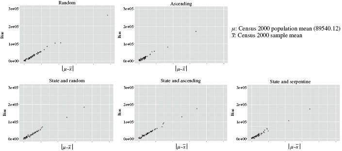
Bias

First, we looked at the relationship between sample balancing and the bias of an estimate. Each graph in Figure 1 shows the relationship between sample balancing and bias of estimates. Bias is defined as the difference between the actual population mean and the estimate \(({{{\hat \mu }_{HT}}})\) from a sample. With regards of the specific sorting method, all 5 graphs indicate that better balancing is associated with a smaller bias.

**Figure 1**  Balancing and bias.

Estimated variance

Figure 2 shows the relationship between balancing and the estimated variance of the U.S. 2010 population mean. In general, a better balanced sample is not necessarily related to a lower estimated variance with the exception of sample selection from the frame with ascending sorting order. The best balanced sample generated slightly larger variance for samples from the frame with ascending sorting order.

**Figure 2**  Balancing and estimated variance.

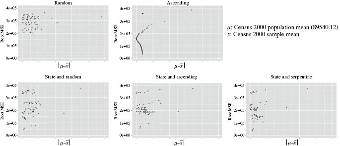
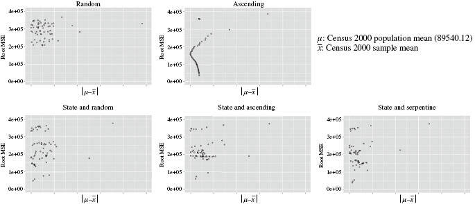
Mean squared error

Figure 3 shows the relationship between balancing and the mean squared error (MSE). MSE is defined as the sum of variance and biased squared. We looked at the MSEs since the bias is exactly known in this simulation. Basically, relationships between balancing and MSE mirrored those between balancing and variance.

**Figure 3**  Balancing and mean squared error.

Conclusion

Our simulation study indicates that a balanced sample is good for reducing bias regardless of the particular sorting method. Rather than selecting a random sample from an ordered frame, we should try to find a balanced sample for an unbiased estimate. However, balanced samples are not necessarily related to smaller variances and MSEs. We should note that a sample is a balanced one if the sample mean of an auxiliary variable is equivalent to the population mean. There could be many ways to obtain the same sample mean. The estimated variance of a sample with the same mean but similar values would be smaller than the estimated variance of a sample with the same mean but vastly differing values. Therefore, it is not surprising to see a larger variance for balanced sample. The interesting relationship between balancing and variance and its functional form in the samples from the frame with an ascending order of Census 2000 population size should be examined further.

Typically, we use available auxiliary variables (e.g., census region, state, metropolitan status, or percent minority) for a sampling design to obtain unbiased and efficient estimates of survey response variables. As discussed, there would be many random samples (equally valid in terms of random selection). But we could find a better sample or more representative sample by utilizing known auxiliary variables. For an area probability sampling design, the U.S. Census tables could be used as useful auxiliary information for balanced samples. Telephone samples also could be evaluated in terms of balance by comparing sample characteristics to the known population characteristics. The current simulation used a highly correlated variable (Census 2000 population size) as an auxiliary variable in estimating the 2010 population size. In practice, it might be difficult to find good auxiliary variables, depending on the specific surveys. In general, it is expected to be beneficial to utilize auxiliary variables as long as the auxiliary variables are moderately correlated to the response variable. Further research is needed in this regard. Only one auxiliary variable was used for the current simulation based on Yates’ definition. A practical balancing approach should be studied further when multiple auxiliary variables are used. Also further research will be pursued applying other balancing methods (e.g., overbalancing ) and/or utilizing auxiliary variable (Census 2000 count in this simulation) as a measure of size for unequal probability samples (Royall and Herson 1973a, 1973b).

Disclaimer and Acknowledgements

The findings and conclusions stated in the manuscripts are solely those of the authors. They do not necessarily reflect the views of the National Center for Health Statistics or the Centers for Disease Control and Prevention. We thank Alan Dorfman for helpful comments and suggestions.