Introduction

As clinical trials move into late phase, real-world research, patients are often surveyed for many years. In other types of sampling, patients are tracked in large insurance claims databases where they are later surveyed. In these studies, the issue of how to handle missing data becomes more important than single surveys because a single missing value will remove a patient from the entire analysis (Graham, Cumsille, and Elek-Fisk 2003; D. Rubin 1987; Tsikriktsis 2005). Missing values complicate the research process at several levels. From the methodological perspective, missing data could represent bias (Seaman and White 2001; Shih 2002). Patients with missing data could be different than those with complete data for many different reasons including demographics, previous therapy, comorbidities, existing conditions and others (Tsikriktsis 2005).

From the research design perspective missing values in repeated measures (within subjects) designs could be handled differently than in group (between subjects) analysis where only a single observation has been made on a smaller number of variables (Graham, Cumsille, and Elek-Fisk 2003; Shih 2002). Additionally, there has been much research from the analytical perspectives including questions regarding the type of imputation (Schlomer, Bauman, and Card 2010) to be made, determination of whether the data is missing at random (D. Rubin 1976; Schlomer, Bauman, and Card 2010), and what percentage of missing data within a variable makes imputation less desirable (Barzi and Woodward 2004; L. Rubin et al. 2007).

The literature demonstrates that mean based imputation is biased (Tsikriktsis 2005). This bias occurs because substituting missing values with a constant decreases the standard deviation. By extension the significance between the two groups will increase. This means the likelihood of incorrectly rejecting the null hypothesis (H_o) increases. This is the definition of Type I error. Similar to mean based imputation, last value carried forward imputation cannot be used in group based analysis as it is a method best suited for repeated measures, and studies have shown it is not accurate (Dinh 2013; Donders et al. 2006; Graham, Cumsille, and Elek-Fisk 2003).

This research introduces distribution based imputation (DBI). DBI works by calculating the mean and standard deviation for a variable that is not missing, and uses those statistics a random distribution of data is simulated. Values from this simulated data are then sampled at random and inserted into the missing values for the real variable. This method is more flexible in databases with a small number of variables were multiple imputation is not possible or ill-advised.

While multiple imputation methods may be shown to be effective in research were a large number of variables with complete data on those variables are available; it would not be applicable in research where only a small number of study variables are used. This research tests DBI against mean based imputation and compares the results against the exact gold standard results that would have been obtained if there were no missing data.

Methods

Data simulations were conducted using the R (sample executable code for performing a simulation is included as an Appendix). To create the simulation, two large distributions (n=100,000) were constructed with the intention of representing the population of values for two variables. These two variables can be thought of as the outcome variable for two independent groups. Simulation instructions for ‘R’ required the X variable to have a mean of 100 and standard distribution (SD) of 15, the second Y variable was instructed to have a mean of 105 and SD also equal to 15. This simulation would then have an overall effect size of 0.33 or 33 percent of one SD.

From these two distributions, four different sample sizes were extracted at random for both the X and Y variables (50, 100, 150, and 200). Within each of the sample sizes, three different missing value percentages were used for each variable (10 percent, 20 percent and 30 percent). This resulted in 12 (4×3) distinct simulations being performed. Missing values for both the distribution and mean imputation methods were selected at random from the given sample size and were the same values within each X and Y array. Imputation methods were performed as follows:

• For mean based imputation, the mean was calculated for the nonmissing data. That mean value was then substituted into the randomly selected places in the array where the missing values had been extracted.
• For DBI, the mean and standard deviation were calculated on the nonmissing data. These values were then used to create a faux-distribution based on 1,000 observations. From this distribution, the number of missing values were extracted without replacement and placed into the array where the missing values had been extracted.

From each of these simulations, three independent t-tests were calculated for the sample sizes mentioned. The first served as the gold standard test and was the result of the X and Y variable with no missing data. The second was the t-test comparing X and Y variables where distribution based imputation had been used, and the third was the t-test comparing X and Y variables where mean based imputation had been used.

Within each sample size and missing value combination (12 simulations), this process was repeated 1,000 times, selecting new samples from the 100,000 X and Y variables at each pass. The means and standard deviations for each of the three conditions (gold standard, distribution imputation, and mean imputation as well as the p-value were written to an external file to facilitate further analysis. This process yielded a master database of 12,000 results specific to all of the conditions mentioned above. Calculation of the t-values and p-values for all of the t-test procedures were performed with the R program t-test procedure, and no test validation was needed.

Data Analysis

From the master database, the number of statistically significant results using a p-value of 0.05 were counted for the gold standard and both distribution and mean imputation methods. The number of rejected (p<0.05) tests were then placed into a table for each of the sample size and missing value percent stratifications and expressed as a percent. The most efficient method is the one that yielded a closer count (percentage) of rejected hypothesis values to the gold standard test. The more unbiased imputation methods would be the one that was both accurate and had counts (percentage) of p-values both above and below the count of the gold standard.

An examination was performed to determine the bias of the imputation method, without regard to the arbitrary cutoff value of p=0.05. In order to examine bias, the calculated value of the p-value was used for both distribution and mean based imputation compared to the gold standard. An unbiased estimator would have approximately the same number of calculated p-values greater than and less than the gold standard p-value. In other words based on 12,000 simulations, an unbiased estimator would have approximately 6,000 calculated p-values both greater than and less than the gold standard p-value. In order for a statistical method to be conclusively determined to be more efficient than another, it must outperform the other method across a variety of different experimental conditions. In this simulation study, the more efficient method is the one that most closely approximates the gold standard values in terms of the absolute number of p-values that would be rejected as well as the percentage of time that the resulting p-value was an over estimate or underestimate of the gold standard p-value.

The last analysis was a descriptive based analysis calculating the average SD value for the X variable across all simulations. This analysis was performed to illustrate the suspicion that using mean based imputation would decrease the SD values, and this then leads to a greater count of statistically significant results and an increase in Type I error.

Results

With regard to the accuracy of the simulation of the population based X and Y values, the results of the R-based population simulation were checked and validated for accuracy (X-variable mean=100.00, SD=14.99. Y-variable mean=105.00, SD=15.01).

Mean based imputation resulted in a higher percentage of rejected HO hypotheses than the gold standard tests in all 12 of the simulation scenarios (100 percent). The range of these differences was less than 1 percent in only two simulations and greater than 5 percent in five of the 12 simulations (Table 1). The average increase in Type I error was 4.57 percent with the smallest increase at 0.2 percent and the greatest increase at 11.6 percent. Five of the simulations yielded increases greater than five percent. Distribution based imputation was not biased as an increase in Type I error was seen in only three of 12 simulations (25 percent). The largest increase in Type I error was only 4.2 percent in a condition where mean based imputation had a Type I error rate of 9.7 percent (n=50, missing 20 percent).

In order to examine the bias of distribution and mean imputation without regard to the alpha level of a statistical test, Table 2 presents the data on the imputation methods based on the calculated value compared to the gold standard. For all of the individual simulations a higher percentage of the mean based imputation, p-values were smaller than the p-values calculated on the gold standard. Across all 12,000 simulations, the p-value for Mean based imputation was greater than the gold standard 3,091 (25.8 percent) of the time and smaller than the gold standard 8,909 (74.2 percent) times. In four of 12 simulations, the p-values were smaller than the gold standard more than 80 percent of the time. This indicates a high level of bias.

For distribution based imputation, there was an even split 50/50 split on one of the 12 simulations which indicates a perfect non-bias condition (n=150, missing 10 percent). The maximum departure from the desired 50 percent value was only 54.6 percent (n=50, missing 20 percent) as compared to 68 percent in the Mean based imputation method. Across all 12,000 simulations Distribution based imputation demonstrated results much closer to the 50/50 results with p-value greater than the gold standard 5,845 (48.7 percent) and p-value less than the gold standard 6,155 (51.3 percent) The difference between distribution and mean based imputation across all 12,000 simulations can be seen graphically displayed in Figure 1.

Figure 1

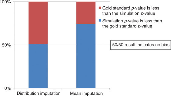
Desired outcome for evidence of no bias is 50/50 split in randomization.

Table 3 displays data regarding the accuracy of the standard deviations for the simulated data on the X variable. Recall that the simulation specification was for a SD=15.00, as can be seen on all occasions the distribution based method of imputation yielded SD values closer to the gold standard and in all occasions the mean based imputation method had SD values that were smaller than the gold standard.

Discussion

In order for a statistical method to be conclusively determined to be more efficient than another, it must outperform the other method across a variety of different experimental conditions. In order to determine bias of an imputation method, the method cannot systematically over or underestimate the gold standard. In this study, DBI was both more efficient and had less bias than mean based imputation.

The fact that mean based imputation had a higher percentage of rejected Ho hypothesis all of the simulation conditions demonstrates a high level of bias for the method. Not only were these percentages higher but in five of the 12 conditions the percentage was more than five percent greater. These percentages are Type I errors and the increase in this error averaged 4.57 percent. This provides clear evidence that mean based imputation is biased. DBI was not biased as the percent of rejections were both higher and lower than the gold standard and averaged only a –1.1 percent which indicates no increase in Type I error when averaged across all simulation conditions.

Similar results were seen when examining the exact, calculated value of the p-value. An unbiased estimate of the gold standard can be determined by and even split of imputated p-values both greater than and less than the gold standard. In this application with 12,000 simulations, a perfect unbiased method would result in 6,000 values both greater and less than the gold standard for a 50/50 split. Distribution based imputation was remarkably close (48.7/51.3) as compared to mean based imputation which was highly biased (25.8/74.2).

The last analysis highlighted in Table 3 displays the reason why mean based imputation leads to more rejected Ho hypothesis. As can be seen in the table the SDs for the mean based imputation are smaller in each of the 12 simulations across all conditions of sample size and missing value percentage. The DBI yields nearly exact SD values as compared to the gold standard. Therefore, the suspicion that the mean based imputation method is biased by the SD being much smaller and leading to a higher or increased Type I error rate is satisfied using the methodology of this study.

Limitations

This study did not address the data missing at random issue. This is more of a research design based issue and would rely on different methods of data analysis or design interpretation. Second, only a limited number of experimental simulations were used in this study and clearly different sample sizes, effect sizes and percentages of missing data could be comprehensively examined. While it is expected that the findings of this study would extend beyond this simulation, it cannot conclusively be determined.

While this study confirms what has been suspected regarding the relative inaccuracy of mean based imputation, it also presents a highly accurate method of imputation that is not biased with regard to that calculated value of the p-value but also highly efficient. The technique of DBI is easy to perform in R and is able to be performed on large datasets regardless of the sample size and percent of missing values within. Whether to use multiple imputation methods or DBI or even no imputation depends on the nature of the experiment and the hypotheses being tested. However, in studies with a smaller number of variables, where other imputation methods cannot be done, DBI is an accurate and unbiased method.

Appendix

Sample code for R that was used to calculate the mean and standard deviation from simulation data and then substitute’s distributional data and substitutes values back to the data. This code can easily be modified to be used on any continuous variable. For detailed instructions, readers may contact the author.

#Create the populational distribution with fixed parameters such as an IQ variable.

xpop<-rnorm(n=100,000, mean=100.0, sd=15)

#Create memory variables for use ‘Pull’ is the number of missing values needed to be pulled from the #simulated data.

n=200

pull=60

#Create the sample one value at a time from the population of 100,000.

for(i in 1:1,000)

x <- sample(xpop,n,replace=F)

xrand <-x

#storing the values to be used in the false distribution to be compared back to simulation for accuracy.

meanx<-mean(x)

sdx<-sd(x)

#selects the numbers that will go into the random replacement.

xselect<-rnorm(1,000,meanx,sdx)

xinsert<-sample(xselect,pull)

#Performs the substitution of the values (60 in this case) that will need to change for each N change.

usexrand<-replace(xrand, c[6:65], xinsert)

meanxrand<-mean(usexrand)

sdxrand<-sd(usexrand)

usexcon<-replace(xconstant, c[6:65], meanx)

meanxcon<-mean(usexcon)

sdxcon<-sd(usexcon)

}

#The next two lines prints the two variables and the reader can see values 6 through 65 have been replaced by the new random variable substitution.

xrand

usexrand