Introduction
Many internet-panels consist of self-selected respondents and hence cover a relatively small part of the population. Estimates based on Internet-panels therefore may suffer from non-coverage and self-selection bias. One way to correct for these biases is to use adjustment weighting (Lee 2006). However, when Internet-panel respondents are intrinsically different from the general population, previous studies showed that weighting may result in an increase in bias (for example, see (Loosveldt and Sonck 2008)).
How can we show that panel-members are intrinsically different from respondents that take part in a conventional random-sample survey? To answer this question we compared the results of a volunteer Internet-panel to the results of a web-interview (WI) based on a random sample of the same population. First, differences in population coverage are studied. Secondly, we test if significant differences in coverage predict differences on dependent variables. Finally, we use propensity matching to test for self-selection bias. This contribution sheds light on the extent of coverage bias relative to self-selection bias in random- and volunteer opt-in Internet surveys.
We use propensity score matching to answer our question. Propensity scores summarize the conditional probability of a respondent to be member of either the random or volunteer sample based on a set of covariates. When the propensity score includes relevant covariates, respondents with the same propensity scores can be matched. Remaining differences between dependent variables after matching cannot be caused by coverage errors, and are indicative for the size of self-selection bias.
Method
The random sample was drawn from a Dutch National data-base of household addresses (Cendris), and included 2500 respondents. These respondents were approached using a two step strategy. Eligible respondents (2025) received an invitation-letter with a log-in code to participate in a Web-Interview (WI). All non-respondents were re-approached by telephone. The WI-sample includes 1347 respondents (AAPOR RR1=0.54). The volunteer Internet-sample was drawn from a larger Internet-panel that used a quota sampling procedure to result in a sample that was representative for the population on gender, job status, and age. The volunteer internet sample consisted of 496 respondents. Reference data for the population were obtained from Statistics Netherlands (2009).
Instruments
This survey was part of a bi-annual governmental monitor on environmental hindrance that has run since 1988. The propensity score was computed using a logistic regression analysis including age, gender, household composition, job status, education and all significant two-way interactions between these variables as covariates and sample membership as dependent variable. As volunteer opt-in panels often consist of ‘engaged citizens’ (Stoop 2005) we also added one motivational variable ‘worrying-about-society’, a composite score of 5 questions on the quality of the Dutch health care system, global environment, safety, industrial pollution, and education to the propensity score (questions measured on a 10-point scale, Cronbach’s alpha=0.70).
As dependent variables we used three variables of which two were composite scores. Environmental hindrance was composed of 7 questions on hindrance from soot dust, stench from industry, stench from traffic, noise from industry, noise from traffic, noise from airplanes, and light pollution (10-point scale, Cronbach’s alpha=0.83), and satisfaction with living environment composed of 4 questions: satisfaction with one’s house, street, neighborhood, and green space (10-point scale, Cronbach’s alpha=0.62). The third variable measures the respondent’s knowledge of the existence of a national telephone number for reporting environmental pollution. We use these dependent variables to compare the samples before and after matching.
Analysis
In this paper we used propensity matching within calipers with the R-program ‘MatchIt’. (D’agostino 1998; Rosenbaum and Rubin 1985). Extensive literature on this software is available in the documentation that comes with the package (Ho et al. 2009). A benefit of caliper matching is that matches are made within a specified maximum distance between propensity scores. Therefore, fewer units will be matched but those matched will be very similar.
Findings
Inspection of Table 1 shows that there are differences in the composition of the samples mutually as well as compared to the Dutch gold standard provided by the Statistics Netherlands (Statistics Netherlands 2009). The differences in composition between the population and the volunteer-panel on age, gender and job status should be very small due to quota sampling. Previous studies found that members of volunteer opt-in panels are usually younger, better educated, and more likely male (Bradley 1999; Kaplowitz, Hedlock, and Levine 2004). Other differences are small but significant, indicating some coverage error.
There are also sample differences on the dependent variables. Internet-panel respondents report significantly more hindrance (p<0.001), less satisfaction with their housing (p<0.01) and more knowledge about the pollution telephone (p<0.001) (see Table 2).
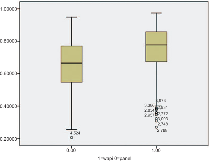
Figure 1 shows the distribution of the propensity to be a respondent in the random WI-sample. Propensities of both distributions vary between 0.2 and 0.98. The mean propensity for the WI sample is 0.78 (0.27 to 0.98) and for the volunteer sample it is 0.68 (0.21 to 0.95). The model explained 30% in the variance between the samples on the included variables. From the figure we can conclude that the two samples overlap considerably, but contain unique respondents as well.

From the overlapping parts of the box-plot, very similar respondents are matched using a caliper size of 0.0005. 178 Respondents from both samples are matched. The matched sample has a balance increase of 99.3%, meaning that the matched respondents share almost the same background characteristics. Therefore, in our matched sample, coverage errors can be excluded as a reason for differences in our dependent variables.
The differences on ‘satisfaction with their housing’ between the WI and volunteer samples seem to disappear after matching as shown in Table 2 (2.13–2.23, t(2,330)=1.94, p>0.05). Before matching, the difference was similar in size, but significant due to increased statistical power (2.10–2.17, t(2,911)=2.85, p<0.01). For this variable, matching was not effective in reducing the size of the difference between the WI and volunteer samples.
For hindrance the results seem clearer. Before matching the difference between both groups is significant (7.95–7.35, t(2,879)=–5.97, p<0.001), for the matched part of the samples the difference becomes smaller although still significant (7.93–7.44, t(2,327)=–2.49, p<0.01).
Finally the large differences that we find before matching on respondents’ knowledge of environmental pollution telephone (0.56–0.39, t(2,871)=–6.24, p<0.001), largely remain as well after matching (0.55–0.36, t(2,332)=–3.80, p<0.01).
Conclusion
Volunteer Internet-panel respondents are not a random part of the general population. Our matching procedure corrected for coverage error, as a result of the matching procedures both matched samples were equal on all variables included in the propensity score. But the matching procedure could not remove the intrinsic differences between the random WI and volunteer Internet panel. Since respondents responded to the exact same survey, these differences cannot be due to mode-effects.
One reason why matching can be unsuccessful is the choice of covariates. We however included the most widely used demographic variables, and added an intrinsic variable that indicates whether someone is an engaged citizen. Both samples do differ on other non-observed variables, which we called intrinsic variables.
Differences in composition between samples can have varying effects for different dependent variables (Duffy et al. 2005). We find some evidence for effect variation across variables, but have to conclude nonetheless that we were not able to correct for differences between a random and volunteer internet sample. We have to conclude that self-selection bias is causing differences between our samples. Further study on the reasons for joining volunteer panels could yield new covariates to include in adjustment procedures. Until we can fully capture the answering process in volunteer panels, statistical solutions can never solve the problem of non-random sampling.
Acknowledgements
Direct comments to: g.lensvelt@uvh.nl. The authors would like to thank TeamVier B.V. for their comments and access to the data used in this paper.