

The Estate Multiplier Technique is an important example of augmentation of a probability sample with a non-probability sample, which is used in practice. The Statistics of Income Division (SOI) of the IRS has for many years used this technique to produce estimates of wealth for the living population from a sample of estate tax return data (ETD) collected primarily for program administration purposes.[1][2] A Federal estate tax return must be filed within 9 months of death for every U.S. decedent whose gross estate equals or exceeds the applicable filing threshold of $675,000 in gross assets for 2001.[3] All of a decedent’s assets, whether owned solely or jointly, and debts are reported on the return. These estimates, although limited by the estate tax filing threshold, provide coverage of the wealthiest 1 to 2 percent of the population that controls between 25 and 30 percent of total U.S. personal wealth.
Estimates of the wealth holdings of the living population are derived by applying a multiplier to the ETD (Mallet 1908). The multiplier m is equivalent to a sampling weight where the probability of selection includes both the probability r of being a decedent and p being included in the SOI sample. Multipliers are calculated separately based on relevant characteristics such as age and gender, denoted by the index a = 1, …, A, and for each SOI sample strata, denoted by the index i = 1, …, I:mai = 1/(ra * pi). Estimated total wealth W = Σ waimai (Atkinson and Harrison 1978, 23).
In practice, the probability that a person will die in a given year is not random; it is conditional on factors such as age, sex, and family history. For the wealthy, additional factors, such as access to better health care, better nutrition, and less hazardous occupations, also play a role (Attanasio and Emmerson 2003). To account for these additional factors, we use mortality probabilities calculated for holders of large dollar value annuity policies as the basis of the multipliers.
One of the strengths of ETD wealth estimates is the large sample size, which supports detailed estimates for relatively small subpopulations. Still, the numbers of very young (under age 40) or very wealthy (gross assets of $5 million or more) decedents tend to vary from year to year and are relatively small in comparison to their representation in the living population. To dampen the effect of these variations, we augment the sample by including returns (all years of death) with these characteristics filed over the 3-year sample period. These segments of the sample then are poststratifed and reweighted to represent the true decedent population for the year of interest.
In addition to augmenting the sample for two “under-sampled” segments of the population, we adjust the multipliers to reduce the effect of outliers on the overall estimates. Following Hansen, Hurwitz, and Madow (1953) we would ideally use post-stratification, but lacking appropriate control totals, the multipliers are instead trimmed to constrain the tails of the net worth distribution to resemble a Pareto distribution, which is often used in wealth and income models. Parameters are drawn from the empirical distribution of net worth implied by Forbes Magazine’s listing of the “400 Richest Americans” for the corresponding year. Using these parameters, estate records with net worth values above the Forbes threshold were divided into net worth categories and the weights trimmed within each. Weights for records with large negative net worth were similarly trimmed.
Evaluating the Estimates
Lacking control totals from a known sampling frame, we evaluate our estimates using independent estimates derived from the Survey of Consumer Finances (SCF). The SCF collects detailed data on respondents’ assets, liabilities, and incomes and provide the best available coverage of the population through its unique sample design.[4] While there are many similarities between the SCF and the ETD, there are important structural differences. First, the SCF is a household survey which uses as its core unit of observation the “primary economic unit,” which consists of an economically dominant single individual or couple (married or living as partners) in a household and all other individuals in the household who are financially interdependent with that individual or couple.[5] The unit of observation for the ETD is always an individual. Second, there are significant differences in sample size and sample variance, with SCF sample size less than 10 percent of the ETD sample for similar population segments. Finally, values reported for tax purposes may be conservative relative to those reported on the SCF, and in some cases, portfolios in the ETD will have been simplified to facilitate consumption needs and eventual transfer of ownership.[6] Thus the SCF suffers more measurement variance while the ETD can suffer more measurement bias.
Despite these differences, the SCF provides the best available data for evaluating the estate multiplier wealth estimates. Focusing on estimates for 2001, the mean age for heads of household in the SCF with assets above $675,000 was 56, and the median age was 54, younger than the ETD, for which mean and median values were 60. We look first at single persons (single, widowed, separated and divorced) since they are defined similarly in both data sets. For this group, the SCF estimates, which are based on only 200 respondents, show relatively close agreement with the ETD estimates for both the number of households and total asset holdings (see Table 1). Estimates of the value of the personal residence were similar for both sources. While financial assets made up larger share of total assets in the EDT estimates (64 percent) than in the SCF (53 percent), the mean and median values were similar for both.
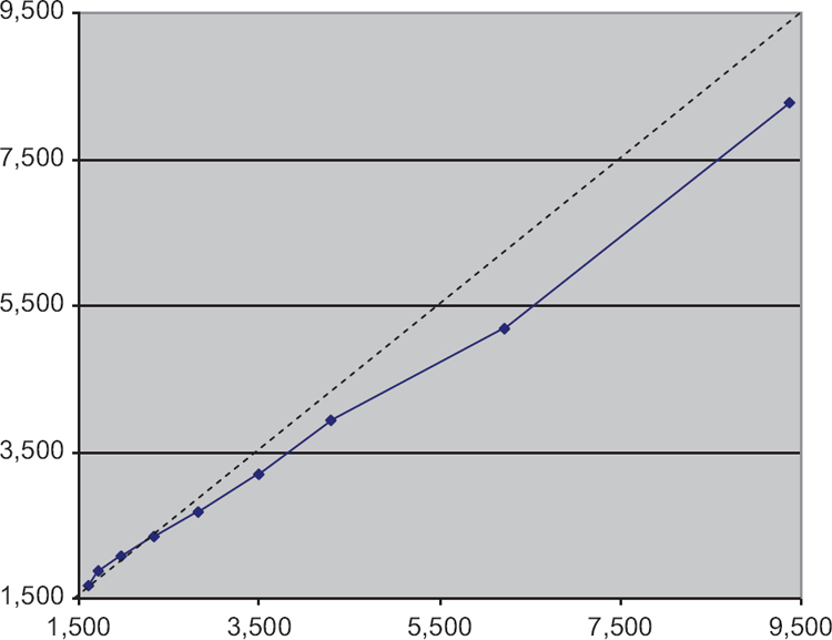
Comparing estimates for married couples in the two data sources raises several challenges. First, married households in the SCF include the assets of both partners while the ETD include only one of a pair and so for comparison purposes, household wealth must be imputed for the ETD.[7] Second, restricting the SCF population to households with $675,000 in total assets, the estate filing threshold, does not completely solve comparability problems because for some SCF households with combined wealth of at least $675,000, both partners’ separate wealth is less. Since similar individuals are missing from the ETD sample, and thus from our imputations, we must account for them in another way. We chose a higher threshold, $1.5 million, to reduce the incidence of this problem. Figure 1 compares the distributions of total assets derived from the SCF and the imputed ETD using a quantile-quantile (QQ) plot.[8] If the underlying distributions implied by the two data sets are similar, the plots will form a straight line and coincide with the 45 degree line. In Figure 1, the plots for the 10th through 90th percentiles are approximately linear and relatively close to the reference line, but with the SCF values somewhat larger than the ETD. The ETD estimate is much higher than the SCF at the 99th percentile (not shown), reflecting the sample variance of both datasets and the difficulty of measuring the extreme tail of the wealth distribution. Overall, these results suggest that the SCF and the imputed ETD produce roughly equivalent measures. It is interesting to note that the mean and median ages for heads of households in the SCF at this higher threshold were 57, virtually the same as for comparable individuals in the ETD.
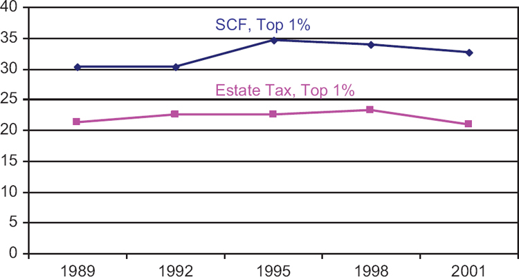
Finally, we examines whether or not the ETD and SCF provide similar estimates of important economic trend, the share of total wealth owned by a fixed portion of the population. The SCF estimates in Figure 2 show that share of wealth owned by the wealthiest one percent of households increased between 1989 and 1995 and then decreased in 1998 and 2001. Estimates of the share of wealth owned by the wealthiest one percent of individuals derived from the ETD, although lower because the data are for individuals rather than households, show a somewhat similar trend, although over all, the ETD estimates are more stable over the entire time period.
Conclusion
The estate multiplier technique is an effective tool that can be used to estimate the wealth for an important segment of the living population using data reported on estate tax returns. The large sample size permits detailed study of demographic groupings, particularly by age, marital status, and sex, characteristics that seem to be key determinants of behaviors such as portfolio choice, charitable giving, and bequest decisions. Estimates for single households in the ETD and SCF were remarkably similar, and our simulations suggest that data for married or partnered households are likewise comparable. In aggregate, both data sets described show similar economic trends. This evidence confirms that wealth estimates derived from tax data provide a useful augmentation to survey data for studying America’s top wealth holders.
Note
The opinions expressed in this paper are the authors’ alone and do not necessary reflect those of the Internal Revenue Service or the Federal Reserve Board of Governors. We are grateful to Arthur Kennickell and Fritz Scheuren for their helpful comments and support of our work.
Annual stratified random samples of estate tax returns incorporate three stratifying variables: year of death, total gross estate combined with certain adjusted taxable gifts (a measure of wealth), and age at death, for a total of 40 strata. Sample rates range from 3 to 100 percent with over half of the strata selected with certainty.
For the most recent estimates, see Raub (2008).
An additional 6-month filing extension is common. Because of this relatively long filing period of up to 13 months, SOI uses a 3-year sample period to ensure complete coverage of a decedent cohort. We make a non-response type adjustment to the sample weights to account for the small number of returns that remain outstanding after the sample period ends.
For a description of the SCF sample, see Kennickell (2007).
For a more complete description of the SCF and recent estimates, see Bucks et al. (2009).
For a detailed discussion of these issues, see Johnson and Moore (2005).
For imputation details, see Johnson and Woodburn (1994).
For a detailed explanation of Q-Q plots see Wilk and Gnanadesikan (1968).